Spatial Data Management
Concepts
Spatial Data
- Location data
- Check-in service
- Online Maps
- Location-based services
- Location tracking
- Traffic Data
Spatial Databases
- PostgreSQL with PostGIS
- Neo4J-spatial
- HadoopGIS
- Ingres
- GeoMesa
Spatial Data Management
- Spatial Database Systems
- Manage large collections of multidimensional objects (2D/3D)
- A spatial object
- Contains (at least) one spatial attributes that describes its location and/or geometry
- A spatial relation
- Is an organized collection of spatial objects of the same entity
Spatial Data
Representation
- Points (Cities in large-scale map)
- Extent (rivers, forest, etc.)
- Vector (approximation by geometric objects)
- Raster (A set of pixels in the grid)
Application
- Spatial data
- GIS
- Segemented images
- Components of CAD constructs or VLSI circuit
- Stars on the sky
- …
- Spatial database
- Users of mobile devices
- Geographers, life scientists
- …
Features of spatial
- Dimensionality
- There is no total ordering of objects in the multidimensional space that preserves spatial proximity
- Complex spatial extent
- No standard definitions of spatial operations and algebra
Relationa indexes (like B+ trees) and query processing methods (sort-merge join, hash-join) are not applicable
Spatial access methods (SAMs) for spatial data have to be defined
- Index spatial objects
- Facilitate efficient processing of simple spatial query types (e.g. range queries)
Spatial Relationships
A spatial relationship associates two objects according to their relative location and extent in space. Sometimes also called "spatial relations".
Can refer to a database relation which stores spatial objects.
Classification
- Topological relationships
- Distance relationships
- Directional relationships
Topological relationships
Each object is characterized by the space it occupies in the universe (A set of pixels).
A set of relationsips between their boundaries and interiors
- Boundary
- Interior (some may not have, points, line segments, etc.)
A hierarchy of relations
- intersect (or overlaps)
- equals
- inside
- contains
- adjacent
- disjoint
Distance relationships
Associate two objects based on their geometric (Euclidean distance), and it’s usually abstracted into human mind.
Distance relationships are expressed either explicitly or by some abstract distance class.
Directional relationships
Associates two object based on their relative orientation according to a global reference system.
Spatial Queries
Applied on one (or more) spatial relations to retrieve objects staisfying some spatial relationships
- Nearest neighbor query
- Spatial join
- Range query
- Spatial selction
- window query
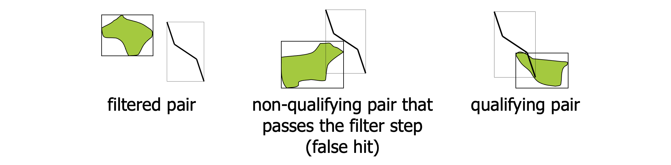
Spatial Query Processing
Evaluating spatial relationships on geometric data is slow.
A spatial object is approximated by its minimum bounding rectangle (MBR)
Process
- Filter: The MBR is tested against the query predicate
- Refinement: The exact geometry of objects that pass the filter step is tested for qualification
Spatial Access Methods (SAMs)
The problem of indexing spatial data
- No dynamic access method with good theoretical worst-case guarantees for range queries
SAMs aim at the minimization of the expected cost.
- Indexing of multidimensional points
Point access methods
Divide the apce into disjoint partitions and group the points according to the regions they belong

Not effective for extended objects (may need to be clipped into several parts which leads to data redundancy and affects performance negatively).
Object clipping can be avoided if we allow the regions of object to overlap.

Optimization
- Group the objects below into 3 groups of 4 objects each such that the MBRs of the groups have the minimum overlap

- Hard optimization problem
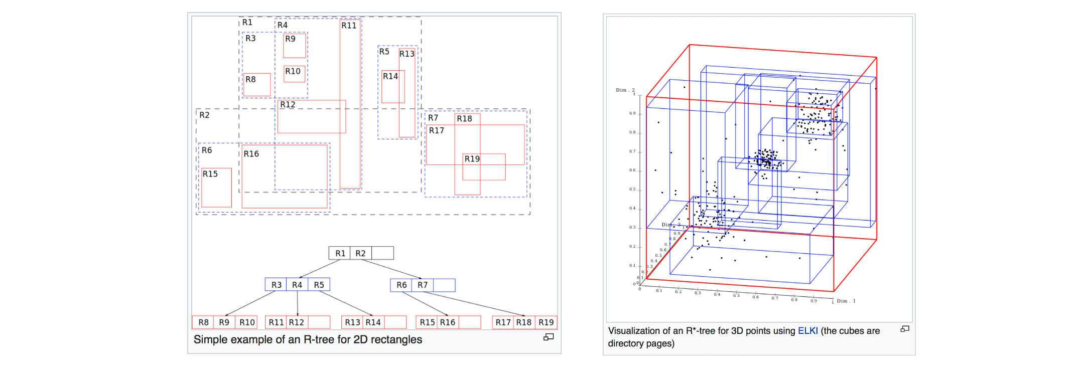
The R-tree
Concept
- Group object MBRs to disk blocks hierarchically
- Each group of object is a leaf of the tree
- The MBRs of the leaf nodes are grouped to form nodes at the next level
- Grouping is recursively applied at each level until a single group (the root) is formed
Elements
- Leaf node entries: <MBR, object-id>, all leaves are in same level
- Non-leaf node entries: <MBR, ptr>, pointing to entries
- Root: have at least two children
- Non-root node parameters
- M
- m
- m <= M/2
- Usually m = 0.4 M
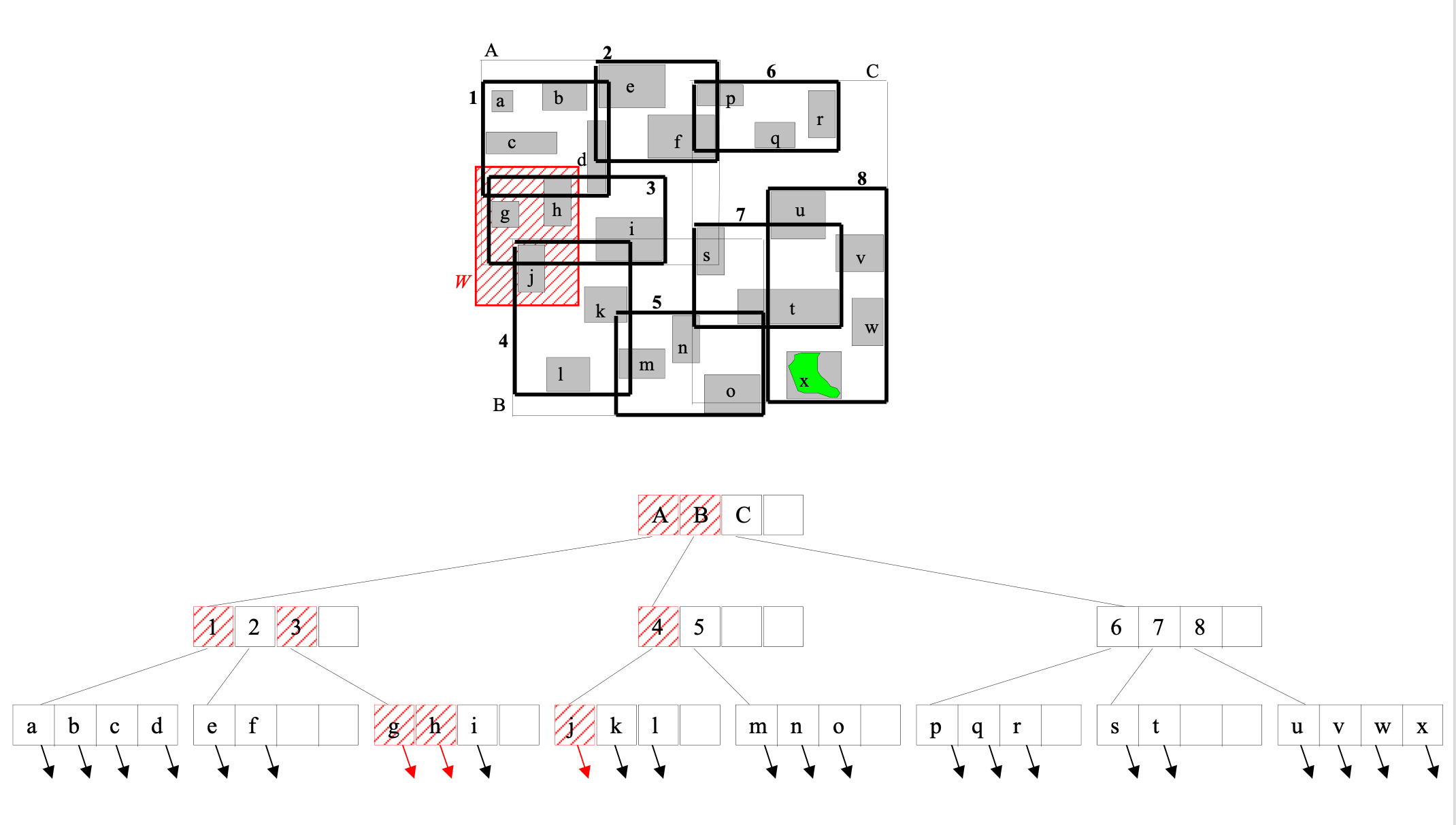
Range searching using an R-tree
Range_query (query W, R-tree node n)
- If n is not a leaf node
- For each index entry e in n such that e.MBR intersects W
- Visit node n’ pointed by e.ptr
- Range_query (W, n’)
- For each index entry e in n such that e.MBR intersects W
- If n is a leaf
- For each index entry e in n such that e.MBR intersects W
- Visit object o pointed by e.object-id
- Test range query against exact geometry of o; If o intersects W, report o
- For each index entry e in n such that e.MBR intersects W
- May follow multiple paths during search
- Different search predicates are used for different realtionships with W
Construction of the R-tree
- Dynamically constructed/maintained
- Insertions/deletions interleave with search operations
- Insertion similiar to B+ Tree, but with special optimization algorithms
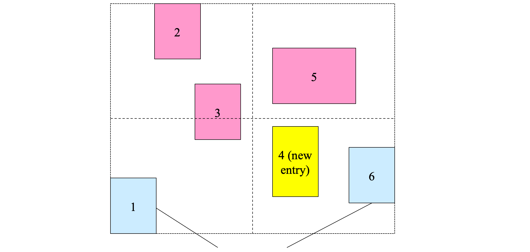
- Choose the path where a new MBR is inserted
- Split overflow nodes
- Underflows in deletions
- Deleting the underflow leaf node
- Re-insert the remaining entries
- Insertion similiar to B+ Tree, but with special optimization algorithms
R*-tree
Only different in the insertion algorithm (compared to R-tree), aiming at constructing a tree of high quality
A good tree
- nodes with small MBRs
- nodes with small overlap
- nodes that look like squares
- nodes as full as possible
Optimization
- Minimize the area covered by an index rectangle (small area means small dead space)
- Minimize overlap between node MBRs (Minimizes the number of traversed paths)
- Minimize the margins of node MBRs (Square-like nodes, smaller number of intersections for a random query, better structure)
- Optimize the storage utilization
- Nodes in tree should be filled as much as possible
- Minimizes tree height and potentially decreases dead space
- Insertion heuristics (Select the path)
- Least MBR enlargement after insertion
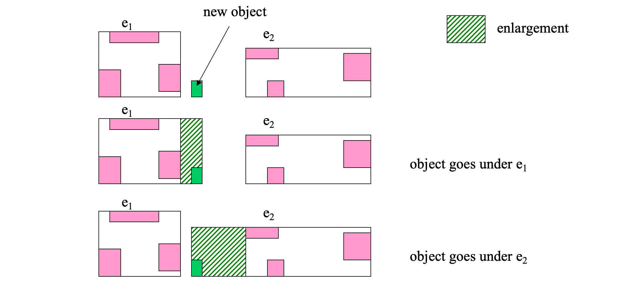
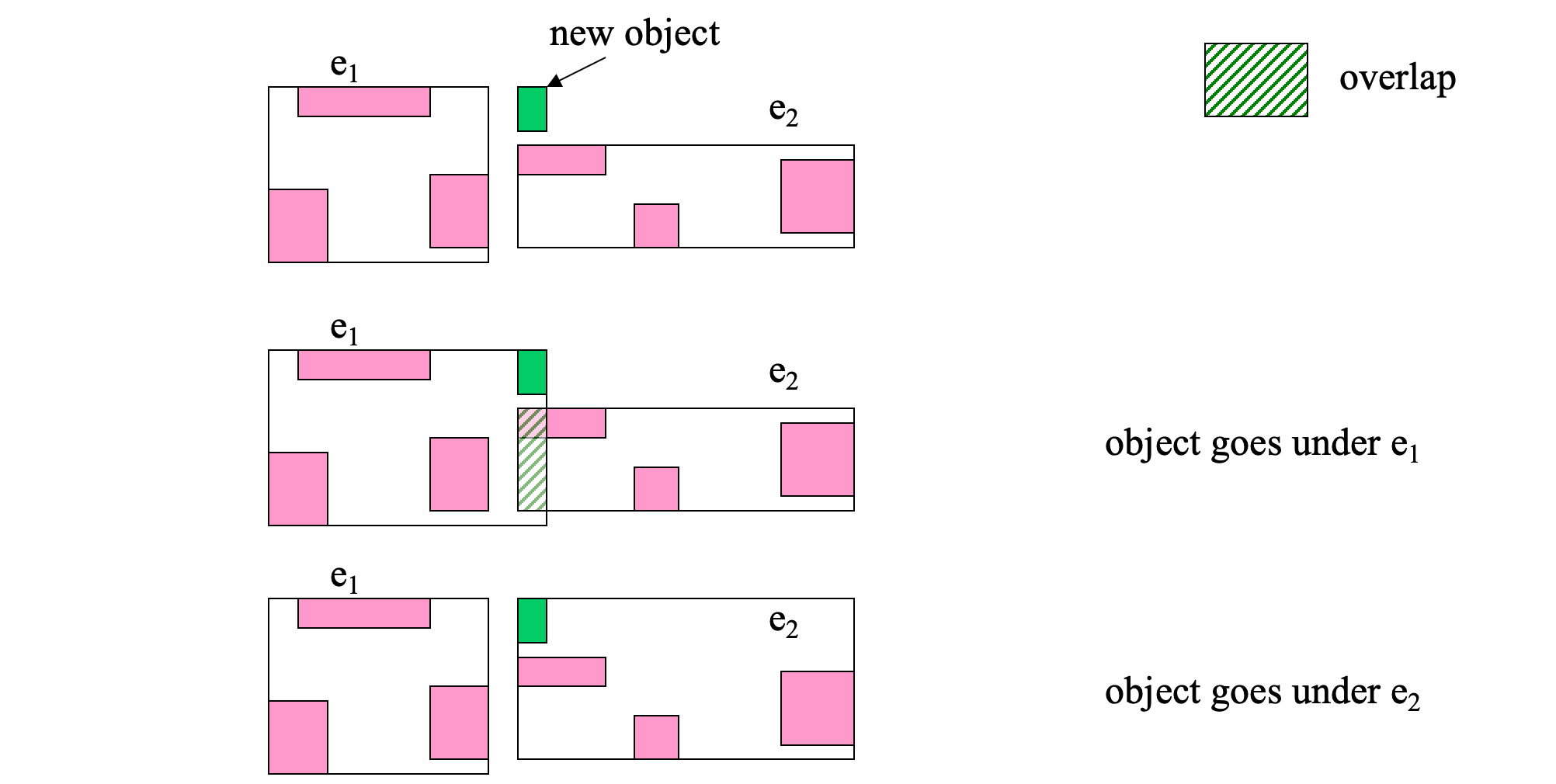
- Least MBR overlap after insertion
- Least MBR enlargement after insertion
Node Spliting
Determine the split axis
- For each axis (i.e. x and y axis)
- Sum=0;
- sort entries by the lower value, then by upper value
- for each sorting (e.g. lower value)
- for k=m to M+1-m
- place first k entries in group A, and the remaining ones in group B
- Sum = Sum + margin(A) + margin(B)
- Choose axis with the minimum Sum
Distribute entries along axis
- Along the split axis, choose the distribution with minimum overlap
- If there are multiple groupings with minimal overlap choose <A,B> such that area(A)+area(B) is minimized
Insertion heuristics: Forced Reinsert
- Forced Reinsert
- When R*-tree node n overflows, instead of splitting n immediately, try to see if some entries in n could possibly fit better in another node
- Find the 30% furthest entries from the center of the group
- Re-insert them to the tree (not to be repeated if another overflow occurs)
- Slightly more expensive, but better tree structure:
- less overlap
- more space is utilized (more full nodes)
Bulk-loading R-trees
Given a static set S of rectangles, build an R-tree that indexes S.
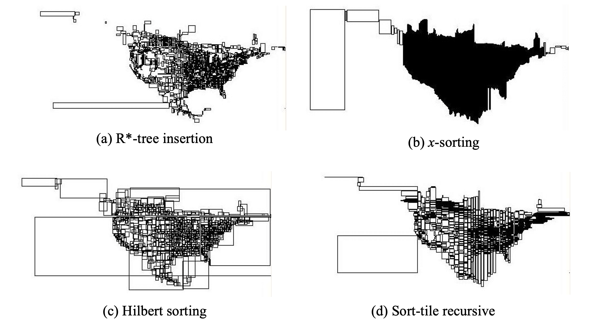
- Method 1: iteratively insert rectangles into an initially empty tree
- Feature
- tree reorganization is slow
- tree nodes are not as full as possible: more space occupied for the tree
- Feature
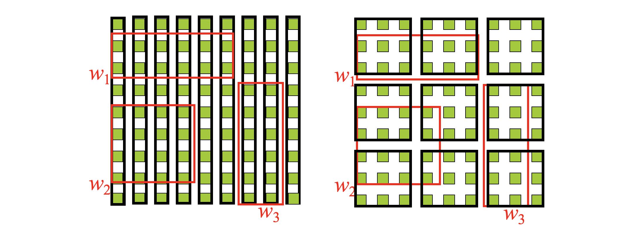
- Method 2 (x-sorting): bulk-load the rectangles into the tree using some fast (sort or hash-based) process
- sort rectangles using the x-coordinate of their center
- pack M consecutive rectangles in leaf nodes
- build tree bottom-up
- Feature
- R-tree is built fast
- good space utilization
- results in leaf nodes that are have long stripes as MBRs
- Method 3 (Hilbert sorting): use a space-filling curve to order the rectangles
- much better structure, but still the nodes have large overlap
- Method 4 (sort-tile-recursive): Sort using one axis first and then groups of sqrt(n) rectangles using the other axis
- Usually the best structure compared to other bulk-loading methods
K Nearest Neighbor Search
Given a spatial relation R, a query object q, and a number k <|R|, find the k-nearest neighbors of q in R.
We can have more than one k-NN sets (with multiple possible equidistant furthest points in them).
Distance measures and MBRs
Distances between MBRs lower-bound the distances between the corresponding objects
dist(MBR(oi),MBR(oj)) ≤ dist(oi, oj)

Distances between R-tree node MBRs lower-bound the distances between the entries in them
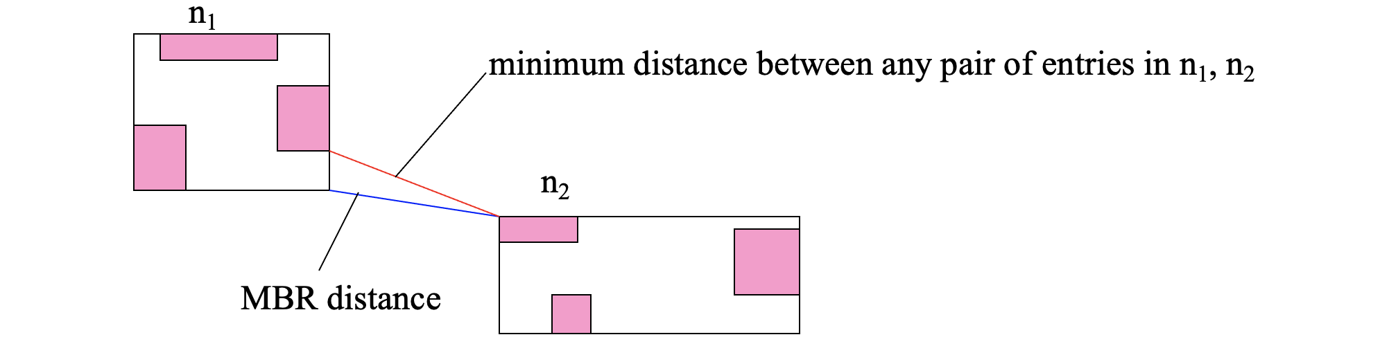
The distance between a query object q and an R-tree node MBR lower-bounds the distances between q and the objects indexed under this node

Depth-first NN search using an R-tree
- Start from the root and visit the node nearest to q
- Continue recursively, until a leaf node nl is visited.
- Find the NN of q in nl.
- Continue visiting other nodes after backtracking as long there are nodes closer to q than the current NN.
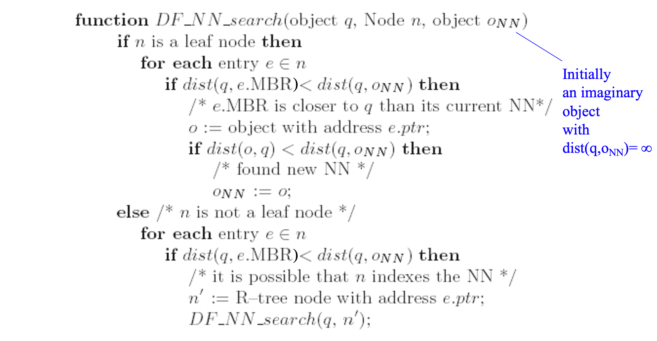
- Large space can be pruned by avoiding visiting R-tree nodes and their sub-trees
- Should order the entries of a node in increasing distance from q to maximize potential for a good NN found fast
- Can be easily adapted for k-NN search
- Requires at most one tree path to be currently in memory – good for small memory buffers
- Characteristic of all depth-first search algorithms
- Recall that the range search algorithm is also DF
- However, does not visit the least possible number of nodes
- Also, not incremental – more on this later…
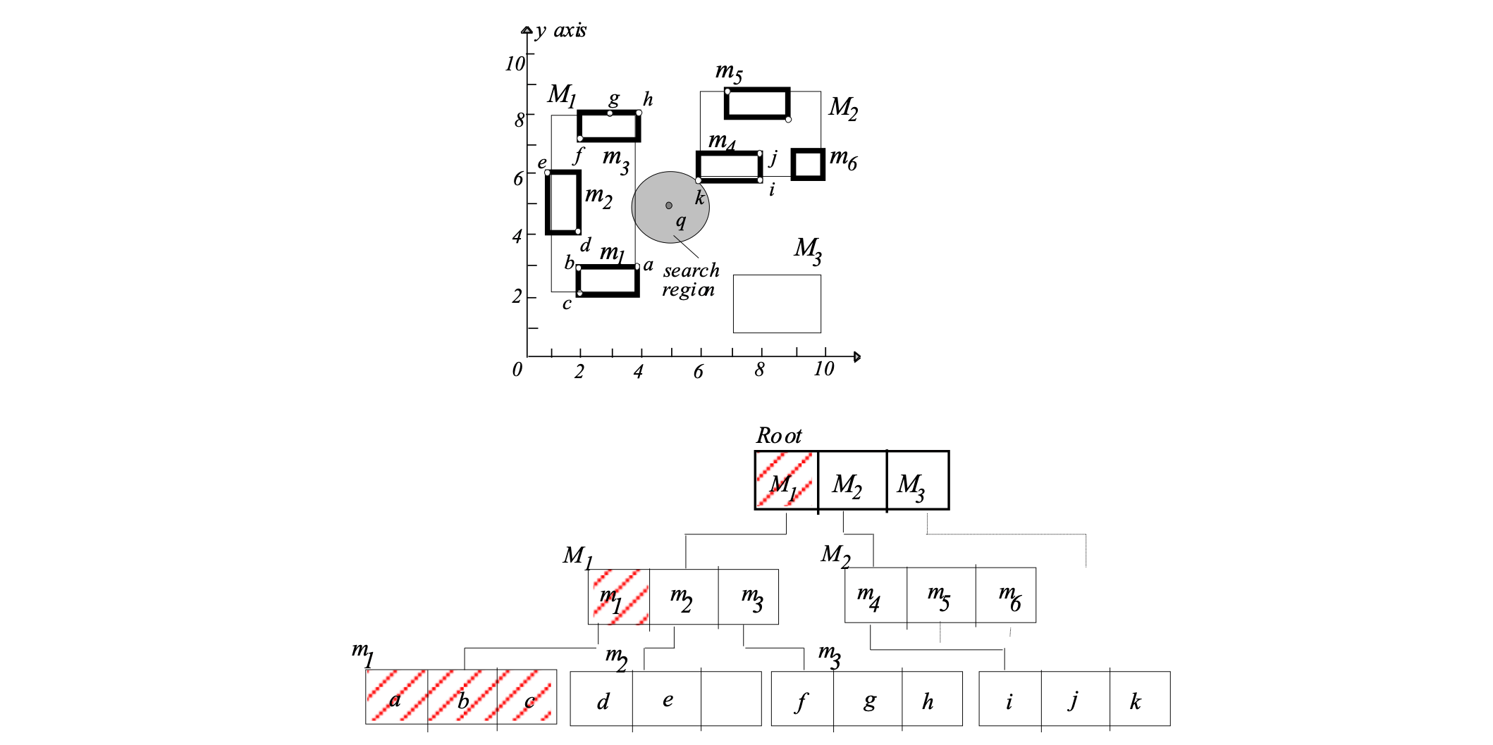
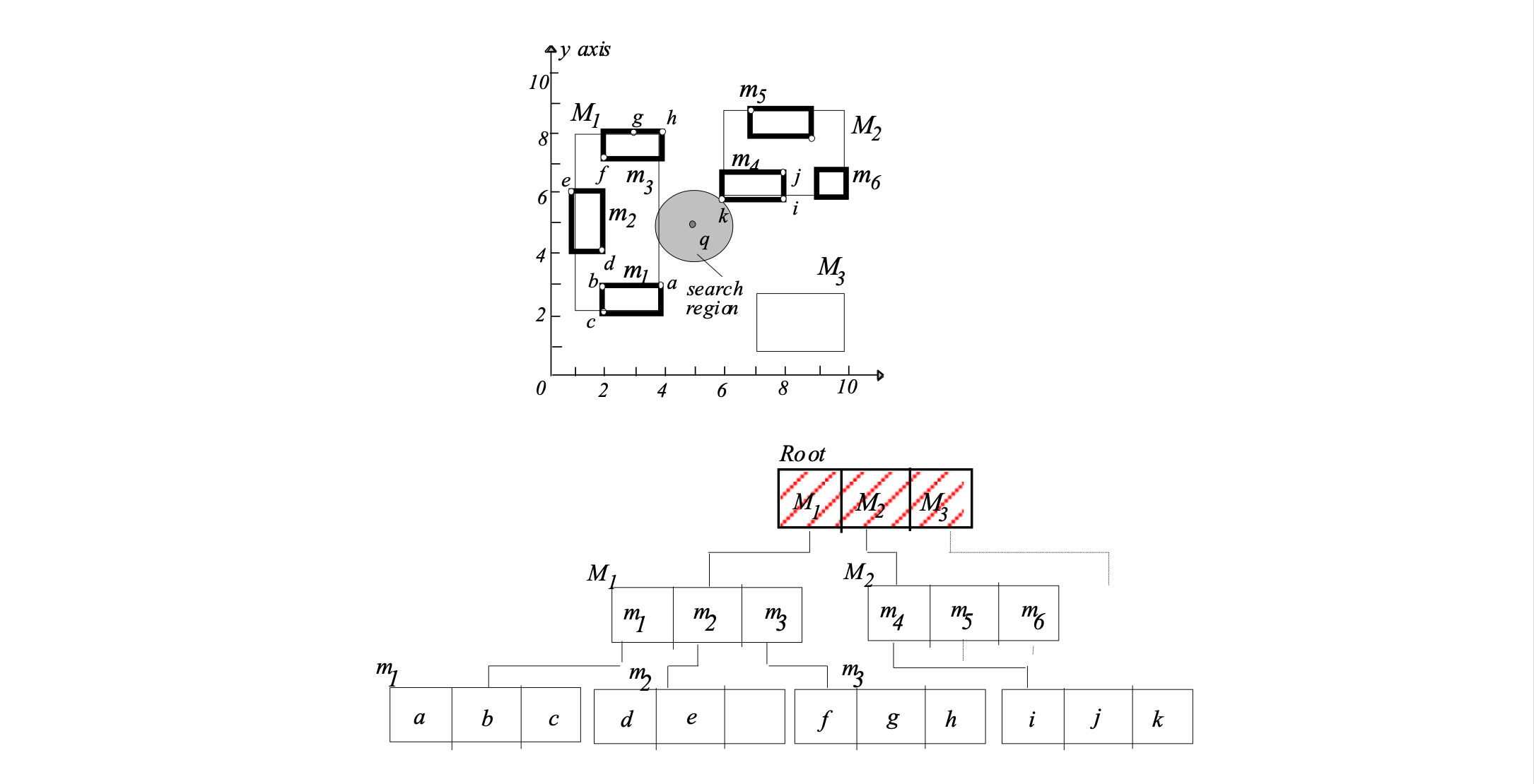
1. visit root
dist(q,M1)<dist(q,oNN)
must visit node M1
2. visit M1
dist(q,m1)<dist(q,oNN)
must visit node m1
3. visit m1
check a,b,c
found new NN:
oNN = a, dist(q,oNN) = sqrt(5)
4. backtrack to M1
check m2
dist(q,m2) = 3 >= sqrt(5):
No need to visit node m2
check m3
dist(q,m3) = sqrt(5) >= sqrt(5):
No need to visit node m3
5. backtrack to root
check M2
dist(q,M2) = sqrt(2) < sqrt(5):
must visit node M2
6. visit M2
check m4
dist(q,m4) = sqrt(2) < sqrt(5):
must visit node m4
7. visit m4
check i,j,k
found new NN:
oNN = k, dist(q,oNN) = sqrt(2)
8. backtrack to M2
check m5
dist(q,m5) >= sqrt(2):
No need to visit node m5
check m6
dist(q,m6) >= sqrt(2):
No need to visit node m6
9. backtrack to root
check M3
dist(q,M3) >= sqrt(2):
No need to visit node M3
10. backtrack from root
Algorithm terminates
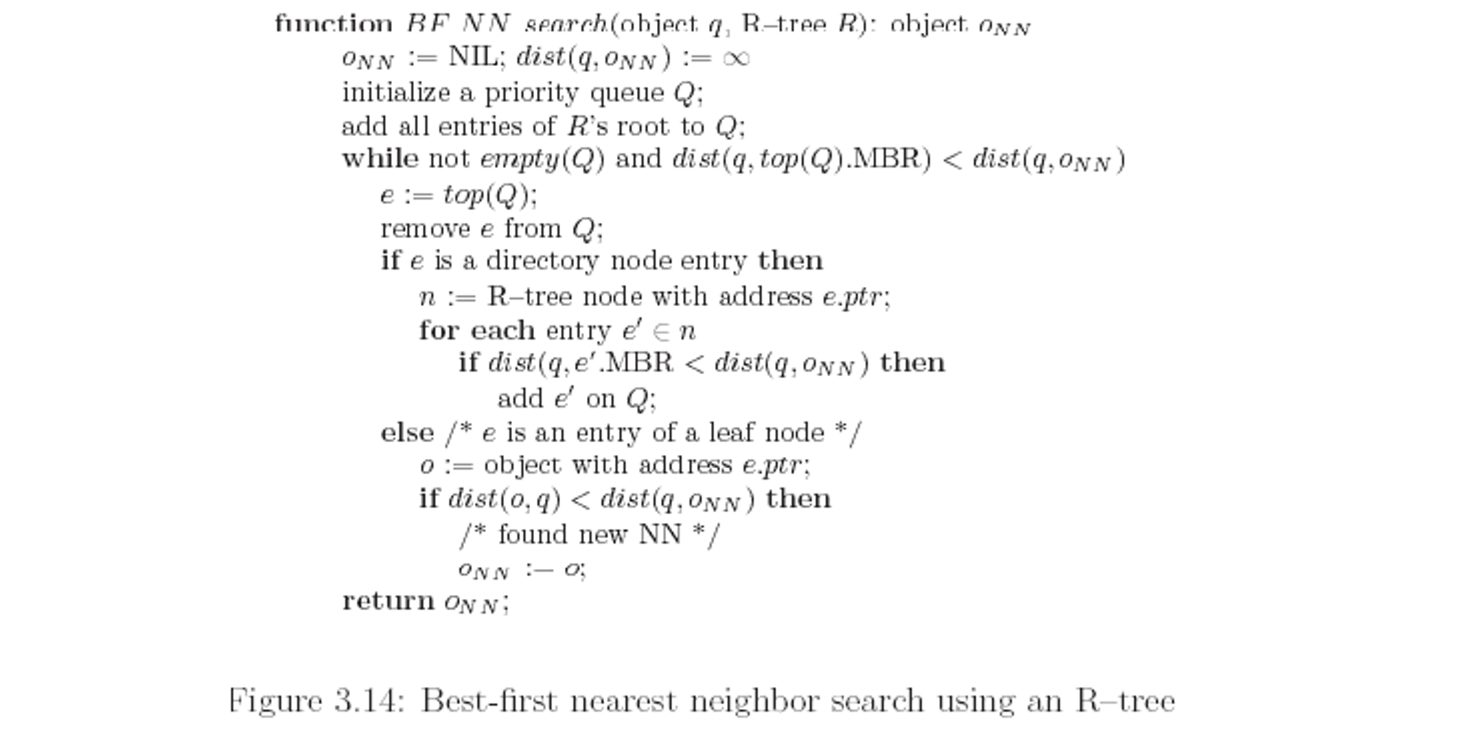
oNN =k with dist(q,oNN)= sqrt(2) foundBest-first NN search
Put all entries in a priority queue and always “open” the closest one, independently of the node that contains it.
Thus the best (i.e., closest) entry is always visited first.
- A more efficient algorithm (given large enough memory)
- Optimal in the number of R-tree nodes visited for a given query q
- Uses a priority queue to organize seen entries and prioritize the next node to be visited
- Adaptable for k-NN search and incremental NN search
- In the previous example, we have visited fewer nodes compared to DF-NN algorithm
- Only nodes whose MBR intersect the disk centered at q with radius the real NN distance are visited (see if you can you prove this)
- The algorithm can be adapted for incremental NN search
- After having found the NN can we easily (incrementally) find the next NN without starting search from the beginning?
- put objects on the heap
- never prune, but wait until an object comes out
- After having found the NN can we easily (incrementally) find the next NN without starting search from the beginning?
- The algorithm can be used for k-NN search
- use a second heap to organize the NN found so far (same can be done for DF-NN)
- no need if we just use the inc. version of the algorithm
- … but: The heap can grow very large until the algorithm terminates
Step 1: put all entries of root on heap Q
Q = M1(1), M2(sqrt(2)), M3(sqrt(8))

Step 2: get closest entry (top element of Q):
M1(1). Visit node M1. Put all entries of
visited node on heap Q
Q = M2(sqrt(2)), m1(sqrt(5)), M3(sqrt(5)), M3(sqrt(8)), m2(3)

Step 3: get closest entry (top element of Q):
M2(sqrt(2)). Visit node M2. Put all entries of
visited node on heap Q
Q =m4(sqrt(2)), m1(sqrt(5)), M3(sqrt(5)), M3(sqrt(8)), m2(3), 	m5(sqrt(13)), m5(sqrt(17))

Step 4: get closest entry (top element of Q):
m4(sqrt(2)). Visit node m4. m4 is a leaf node, so update NN if some object in m4 is closer than the current NN:
oNN = k, dist(q,oNN)= sqrt(2)
Q =m1(sqrt(5)), M3(sqrt(5)), M3(sqrt(8)), m2(3), 	m5(sqrt(13)), m5(sqrt(17))

Step 5: get closest entry (top element of Q):
m1(sqrt(5)). Since sqrt(5) >= dist(q,oNN)= sqrt(2), search stops and oNN is returned as the NN of q
incremental NN search
- Example 1: find the nearest large city (>10,000 residents) to my current position
- Solution 1:
- find all large cities
- apply NN search on the result
- could be slow if many such cities
- also R-tree may not be available for large cities only
- Solution 2:
- incrementally find NN and check if the large city requirement is satisfied; if not get the next NN
- Solution 1:
- Example 2: find the nearest hotel; see if you like it; if not get the next one; see if you like it; …
Spatial Joins
Most algorithms focus on the efficient processing of the filter step.
Most spatial predicates on actual objects reduce to intersection of MBRs in the filter step. Thus all algorithms consider mainly the intersect predicate.
Types
- intersection joins
- Semi-join: Find the cities that intersect a river
- Similarity join: Find pairs of hotels, restaurants close to each other (with distance smaller than 100m)
- Closest pairs: Find the closest pair of hotels, restaurants
- All-NN: For each hotel find the nearest restaurant
- Iceberg distance join: Find hotels close to at least 10 restaurants
Three categories of spatial join algorithms
- Both inputs are indexed (e.g., synchronized tree traversal)
- One input is indexed (e.g., indexed nested loops)
- Neither input is indexed (e.g., spatial hash join)
R-tree (Intersection) Join
Applies on two R-trees of spatial relations R and S
Node MBRs at the high level of the trees can prune object combinations to be checked
This pseudo-code version assumes that the trees have same height
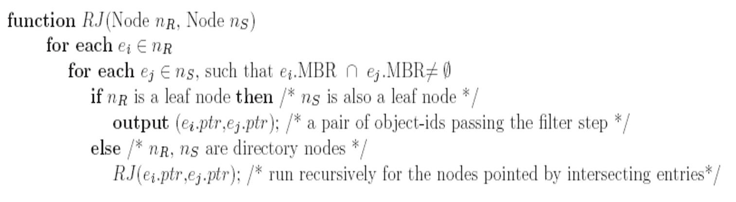
Example
- run for root(RA), root(RB)
- for every intersecting pair there (e.g., A1, B1) run recursively for pointed nodes
- intersecting pairs of leaf nodes are qualifying object MBR pairs
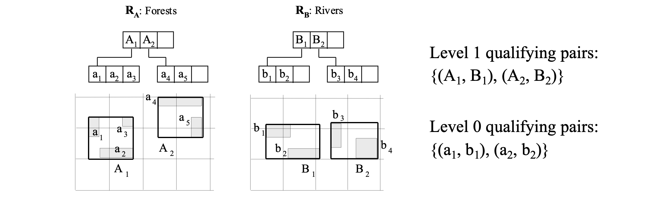
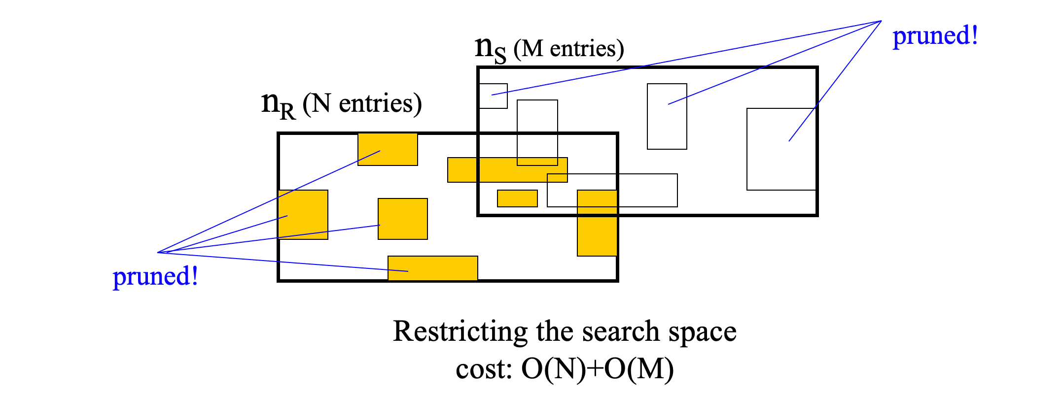
Optimization
space restriction
- If an entry in n1 does not intersect the MBR of n2 it may not intersect any entry in n2.
- Perform two scans in n1 and n2 to prune such entries
plane sweep
- Sort entries in both nodes on their lower-x value (lower bound of x-projection)
- Sweep a line to find fast all entry pairs that qualify x-intersection
- for each of them check y-intersection
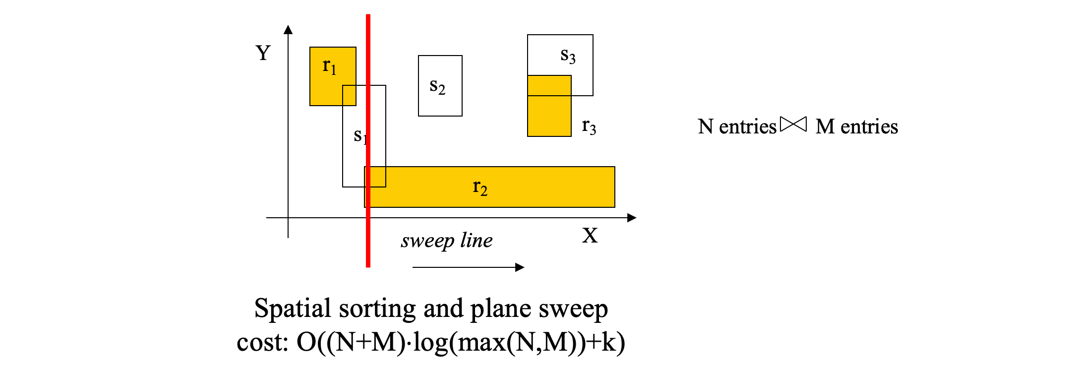
- Worst-case sub-optimal. But very effective on the average
- Worst-case optimal algorithms require advanced data structures for y-intersection. Large hidden constants, thus high cost for this problem size
- Can be used with other spatial join algorithms
R-tree join
- The most efficient algorithm (assuming that the relations are indexed)
- Cannot be used for non-indexed inputs
- unless we build on-the-fly R-trees
- Comes with some I/O scheduling techniques for minimizing the page accesses
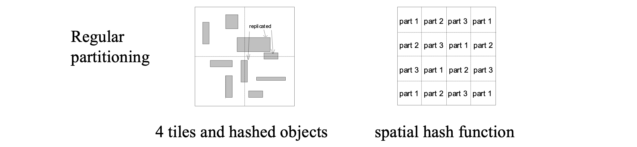
Joining non-indexed inputs
Spatial hash join
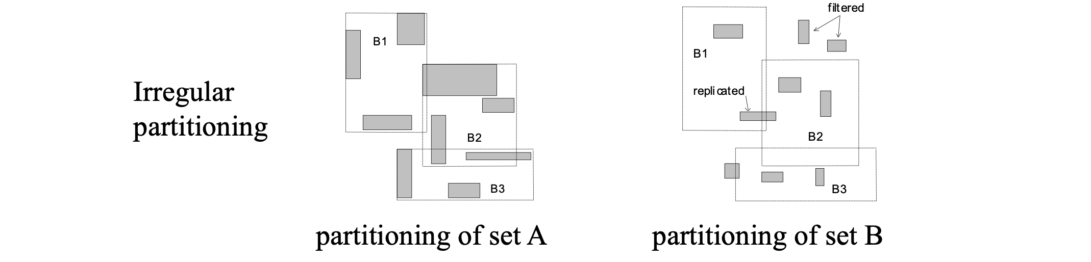
Partition based spatial merge join
Indexed Nested Loops

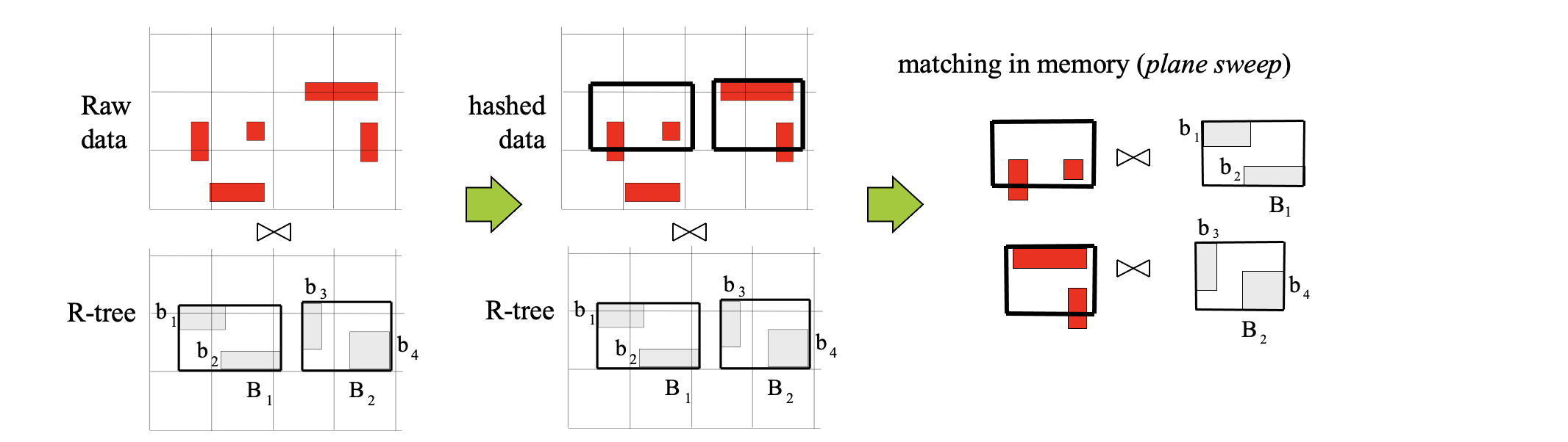
Seeded tree join and Bulk-load and Match build an on-the-fly R-tree

Slot-index spatial join applies hash-join using the entries of a high R-tree level
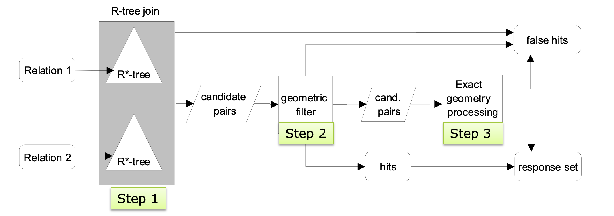
The refinement step
- Step 1: find MBR pairs that intersect
- Step 2: compare some more detailed approximations to make conclusions (a.k.a. geometric filter)
- conservative approximations
- e.g., convex hull
- progressive approximation
- e.g., maximum enclosed rectangle
- conservative approximations

- Step 3: if still join predicate inconclusive, perform expensive refinement step
- can be processed by computational geometry algorithms
- Multi-step processing (R-tree join as example)