COMP7404 Computational Intelligence and Machine Learning

Topic 1 Solving Problems by Searching

Types of Search

Uninformed Search (Know nothing about the problem except definition)
Informed Search (know something more like how close to the goal)
Local Search (Randomly initilize a state and make it better, e.g. Deep Learning)
Constraint Satisfaction Problems (Know more about the problem)
Adversarial Search (have an opponent, e.g. chess, star craft game)

Is Search the same as Unsupervised/Supervised Learning?

Search is a process that tries to explore all options and find out which one is best. Search itself isn’t considered as Machine Learning though it’s always combined with Machine Learning in some system to improve the performance. Machine Learning is part of Artificial Intelligence.

Search Applications

Vacuum World
Pancake Flipping
8 Puzzle
Pathing
TSP
Game Play (chess, Go)

Any problem where more than one alternative needs to be explored may try search

Search Problem Definition

States - Agent location, dirt location
Initial State
Actions and Transition Model
- available possible actions
- what each action does
Goal Test
Path Cost

A solution is a sequence of actions which transforms the start state to a goal state

State Space (the set of all reachable states)

Usually a graph
The possible action sequences form a search tree

State Space Graph vs. Search Tree

State Space Graph (each state occurs only once)
- Nodes - states
- Arcs (connections between nodes) - action results
- A set of goal nodes - goal test
Search Tree (states may occur more than once)
- Root - start state
- Nodes - possible action sequences

some related concepts:

depth of tree
branching factor (max children)

States vs. State Sequence

A large number of state space -> A huge number of state sequences (e.g. a large number of nodes in the search tree)

Example: Chess (10^43 possible states and 10^120 possible state sequences)

Romania Problem

States
- The cities
Initial State
- Arad
Actions and Transition model
- Go to neighboring city
Goal Test
- In Bucharest?
Path Cost
- Distance between the cities

romania_problem

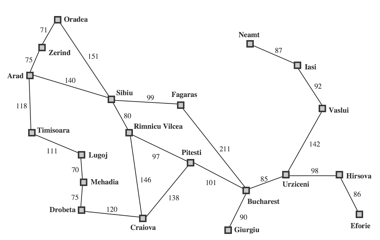
Store data in Python dictionary

romania = {
    'A':['S','T','Z'],'Z':['A','O'],'O':['S','Z'],'T':['A','L'],'L':['M','T'],'M':['D','L'],
    'D':['C','M'],'S':['A','F','O','R'],'R':['C','P','S'],'C':['D','P','R'],
    'F':['B','S'],'P':['B','C','R'],'B':[]
    }

Use dictionart to store neighbors for each cities

>>> romania['A']
['S', 'T', 'Z']

Search Strategy

Defines the order of node expansion
Evaluated along the following dimensions
- Completeness (always find a solution if exists)
- Optimality (find a least-cost solution)
- Time complexity (number of nodes generated)
- Space complexity (max number of nodes in memory)

Time/Space complexity

b: maximum branching factor of the search tree
d: distance to root of the shadowest solution
m: maximum length of any path in the state space

Search Algorithms

~~Tree search algorithm~~ (TSA)
~~Graph search algorithm~~ (GSA)

Uninformed (Blind) Search Strategies

Breadth-first search (BFS)
- BFS-TSA
- BFS-GSA
Depth-first search (DFS)
- DFS-TSA
- DFS-GSA
Uniform-cost search (UCS)
- UCS-TSA
- UCS-GSA

BFS (Time and Space Complexity)

Time - O(b^(d+1))
Space - O(b^(d+1))

DFS (Space Complexity)

Time - O(b^m)
Space - O(m*b)

UCS (Time and Space Complexity)

O(b^(C*/epsilon))

C*: cost of the optimal solution

epsilon: smallest path cost

Queue

Use deque in Python3

    class collections.deque([iterable[, maxlen]])
    Returns a new deque object initialized left-to-right (using append()) with data from iterable.
    If iterable is not specified, the new deque is empty.

>>> import collections
>>> queue = collections.deque(['A', 'B', 'C', 'D'])
>>> queue.popleft()
'A'
>>> queue
deque(['B', 'C', 'D'])
>>> queue.popleft()
'B'
>>> queue
deque(['C', 'D'])

TSA - BFS Version

When it applies DFS/UCS, only need to change the data type of the frontier variable.

pseudo code

    function TSA(problem) returns solution
        initialize frontier using initial state of problem
        while frontier is not empty
            choose a node and remove it from frontier
            if node contains a goal state then return corresponding solution
            explore the node, adding the resulting nodes to the frontier

actual python code

import collections
def bfsTsa(stateSpaceGraph, startState, goalState):
    frontier = collections.deque([startState])
    while frontier:
        node = frontier.popleft()
        if (node.endswith(goalState)): return node
        for child in stateSpaceGraph[node[-1]]: frontier.append(node+child)

My demo of this bfsTsa.py

GSA - BFS Version

pseudo code

    function GSA (problem) returns solution
        initialize frontier using initial state of problem
        initialize explored set to be empty
        while frontier is not empty
            choose a node and remove it from frontier
            if node contains a goal state then return corresponding solution
            If node is not in explored set
                add node to explored set
                explore the node, adding the resulting nodes to the frontier

actual python code

import collections
def bfsGsa(stateSpaceGraph, startState, goalState):
    frontier = collections.deque([startState])
    exploredSet = set()
    while frontier:
        node = frontier.popleft()
        if (node.endswith(goalState)): return node
        if node[-1] not in exploredSet:
            exploredSet.add(node[-1])
            for child in stateSpaceGraph[node[-1]]: frontier.append(node+child)

My demo of this bfsGsa.py

DFS

DFS explores the deepest node in the search tree

Stack

>>> import collections
>>> queue = collections.deque(['A', 'B', 'C', 'D'])
>>> queue.pop()
'D'
>>> queue
deque(['A', 'B', 'C'])
>>> queue.pop()
'C'
>>> queue
deque(['A', 'B'])

TSA - DFS Version

import collections
def dfsTsa(stateSpaceGraph, startState, goalState):
    frontier = collections.deque([startState])
    while frontier:
        node = frontier.pop()
        if (node.endswith(goalState)): return node
        print('Exploring:',node[-1],'...')
        for child in stateSpaceGraph[node[-1]]: frontier.append(node+child)

No results due to revisiting already explored nodes

My demo of this dfsTsa.py

GSA - DFS Version

import collections
def dfsGsa(stateSpaceGraph, startState, goalState):
    frontier = collections.deque([startState])
    exploredSet = set()
    while frontier:
        node = frontier.pop()
        if (node.endswith(goalState)): return node
        if node[-1] not in exploredSet:
            exploredSet.add(node[-1])
            for child in stateSpaceGraph[node[-1]]: frontier.append(node+child)

My demo of this dfsGsa.py

Choices of Search Algorithms

BFS vs DFS
- Don’t use BFS when b (maximum branching factor) / d (distance to root of the shadowest solution) is big
- Don’t use DFS when m (maximum length of any path) is big
- Choose BFS is solution is close to the root of tree
- Choose DFS is solution is deep inside the search tree
TSA vs GSA
- TSA (only frontier)
  - Could stuck in infinite loops
  - Explore redundant loops
  - Require less memory
  - Easier to implement
- GSA (froniter + explored set)
  - Avoid infinite loops
  - Eliminate many redundant paths

Both have time complexity issue

UCS (Cheapest First Search)

Explores the cheapest node first

romania = {
'A':[(140,'S'),(118,'T'),(75,'Z')],'Z':[(75,'A'),(71,'O')],'O':[(151,'S'),(71,'Z')],
'T':[(118,'A'),(111,'L')],'L':[(70,'M'),(111,'T')],'M':[(75,'D'),(70,'L')], 'D':[(120,'C'),(75,'M')],'S':[(140,'A'),(99,'F'),(151,'O'),(80,'R')], 'R':[(146,'C'),(97,'P'),(80,'S')],'C':[(120,'D'),(138,'P'),(146,'R')], 'F':[(211,'B'),(99,'S')],'P':[(101,'B'),(138,'C'),(97,'R')],'B':[]}

Priority Queue in Python (Use heapq in Python3)

frontier = []
>>> from heapq import heappush, heappop
import random
>>> heappush(frontier, (random.randint(1, 10), 'A'))
>>> heappush(frontier, (random.randint(1, 10), 'B'))
>>> heappush(frontier, (random.randint(1, 10), 'C'))
>>> frontier
[(2, 'C'), (7, 'B'), (6, 'A')]
>>> heappop(frontier)
(2, 'C')
>>> heappop(frontier)
(6, 'A')
>>> heappop(frontier)
(7, 'B')
>>> (1, 'B') < (2, 'A')
True
>>> (1, 'B') < (1, 'A')
False

TSA - UCS Version

from heapq import heappush, heappop
def ucsTsa(stateSpaceGraph, startState, goalState):
    frontier = []
    heappush(frontier, (0, startState))
    while frontier:
        node = heappop(frontier)
        if (node[1].endswith(goalState)): return node
        for child in stateSpaceGraph[node[1][-1]]:
            heappush(frontier, (node[0]+child[0], node[1]+child[1]))

GSA - UCS Version

from heapq import heappush, heappop
def ucsGsa(stateSpaceGraph, startState, goalState):
    frontier = []
    heappush(frontier, (0, startState))
    exploredSet = set()
    while frontier:
        node = heappop(frontier)
        if (node[1].endswith(goalState)): return node
        if node[1][-1] not in exploredSet:
            exploredSet.add(node[1][-1])
            for child in stateSpaceGraph[node[1][-1]]:
                heappush(frontier, (node[0]+child[0], node[1]+child[1]))

Informed Search

Employ problem specific knowledge beyond the definition of the problem itself

Heuristic function

Example

Greedy best-first search
A* search

Heuristic Function (designed for a particular search problem)

A function that estimate how close you are to the goal

h(n)

Cost of the cheapest path from the state at node n to a goal state
If n is a goal node, h(n) = 0

Greedy Search (Best-first Search)

Expand the node that has the lowest h(n)

Updated Romania Problem Definition (Add h(n))

romaniaH = {
    'A':366,'B':0,'C':160,'D':242,'E':161,'F':176,'G':77,'H':151,'I':226,
    'L':244,'M':241,'N':234,'O':380,'P':100,'R':193,'S':253,'T':329,'U':80,
    'V':199,'Z':374}

Greedy TSA Practice

from heapq import heappush, heappop
def greedyTsa(stateSpaceGraph, h, startState, goalState):
    frontier = []
    heappush(frontier, (h[startState], startState))
    while frontier:
        node = heappop(frontier)
        if (node[1].endswith(goalState)): return node
        for child in stateSpaceGraph[node[1][-1]]:
            heappush(frontier, (h[child[1]], node[1]+child[1]))

A* Motivation UCS-TSA

orders by backward cost

g(n)

A* Motivation Greedy-TSA

orders by forward cost

h(n)

* always means optimal in AI

A* Motivation A*-TSA

orders by backward cost + forward cost

f(n) = g(n) + h(n)

A*-TSA Practice

from heapq import heappush, heappop
def aStarTsa(stateSpaceGraph, h, startState, goalState):
    frontier = []
    heappush(frontier, (h[startState], startState))
    while frontier:
        node = heappop(frontier)
        if (node[1].endswith(goalState)): return node
        for child in stateSpaceGraph[node[1][-1]]:
            heappush(frontier, (node[0]+child[0]-h[node[1][-1]]+h[child[1]], node[1]+child[1]))
aStarMotivation = {
'S':[(1,'a')],'a':[(1,'b'),(3,'d'),(8,'e')],'b':[(1,'c')],'c':[],'d':[(2,'G')],'e':[(1,'d')]}
aStarMotivationH = {'S':6,'a':5,'b':6,'c':7,'d':2,'e':1,'G':0}

Admissibility of Heuristic

A heuristic h(n) is admissible (optimistic)

1 <= h(n) <= h(n)*

where h*(n) is the true cost of the nearest goal

Optimality of A*

A* is optimal if an admissible heuristic is used

Consistency of Heuristic

Definition
- Heuristic cost <= actually cost for each arc
  - h(a) - h(c) <= cost (a to c)
Consequence of consistency
- The f value along a path never decrease
  - h(a) <= cost(a to c) + h(c)

2020-11-11

xDeepFM for Recommender Systems - 推荐系统

2020-10-05

COMP7404 Topic 3 Adversarial Search

2020-10-04

COMP7404 Topic 2 Beyond Classical Search