Background
Network Distance
- In many real applications accessibility of objects is restricted by a spatial network
- Examples
- Driver looking for nearest gas station
- Mobile user looking for nearest restaurant
- Examples
- Shortest path distance used instead of Euclidean distance
- SP(a,b) = path between a and b with the minimum accumulated length
Challenges
- Euclidean distance is no longer relevant
- R-tree may not be useful, when search is based on shortest path distance
- Graph cannot be flattened to a one-dimensional space
- Special storage and indexing techniques for graphs are required
- Graph properties may vary
- directed vs. undirected
- length, time, etc. as edge weights
Modeling and Storing Spatial Networks
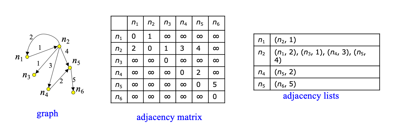
Modeling Spatial Networks
- Adjacency matrix only appropriate for dense graphs
- Spatial networks are sparse: use adjacency lists instead
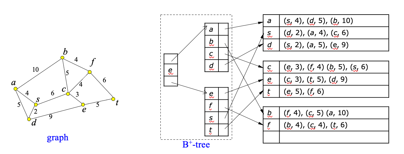
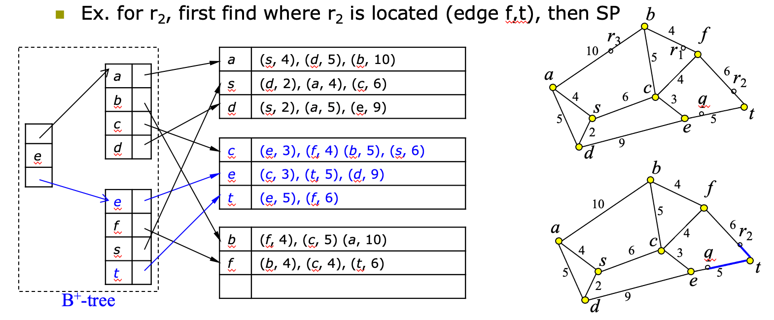
Storing Large Spatial Networks
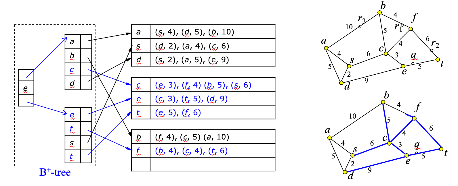
- Problem: adjacency lists representation may not fit in memory if graph is large
- Solution:
- partition adjacency lists to disk blocks (based on proximity)
- create B+-tree index on top of partitions (based on node-id)
Shortest Path Search
- Given a graph G(V,E), and two nodes s,t in V, find the shortest path from s to t
- A classic algorithmic problem
- Studied extensively since the 1950’s
- Several methods:
- Dijkstra’s algorithm
- A*-search
- Bi-directional search
Dijkstra’s Shortest Path Search
- idea: incrementally explore the graph around s, visiting nodes in distance order to s until t is found (like NN)
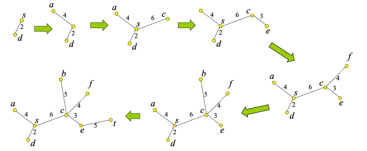
Algorithm
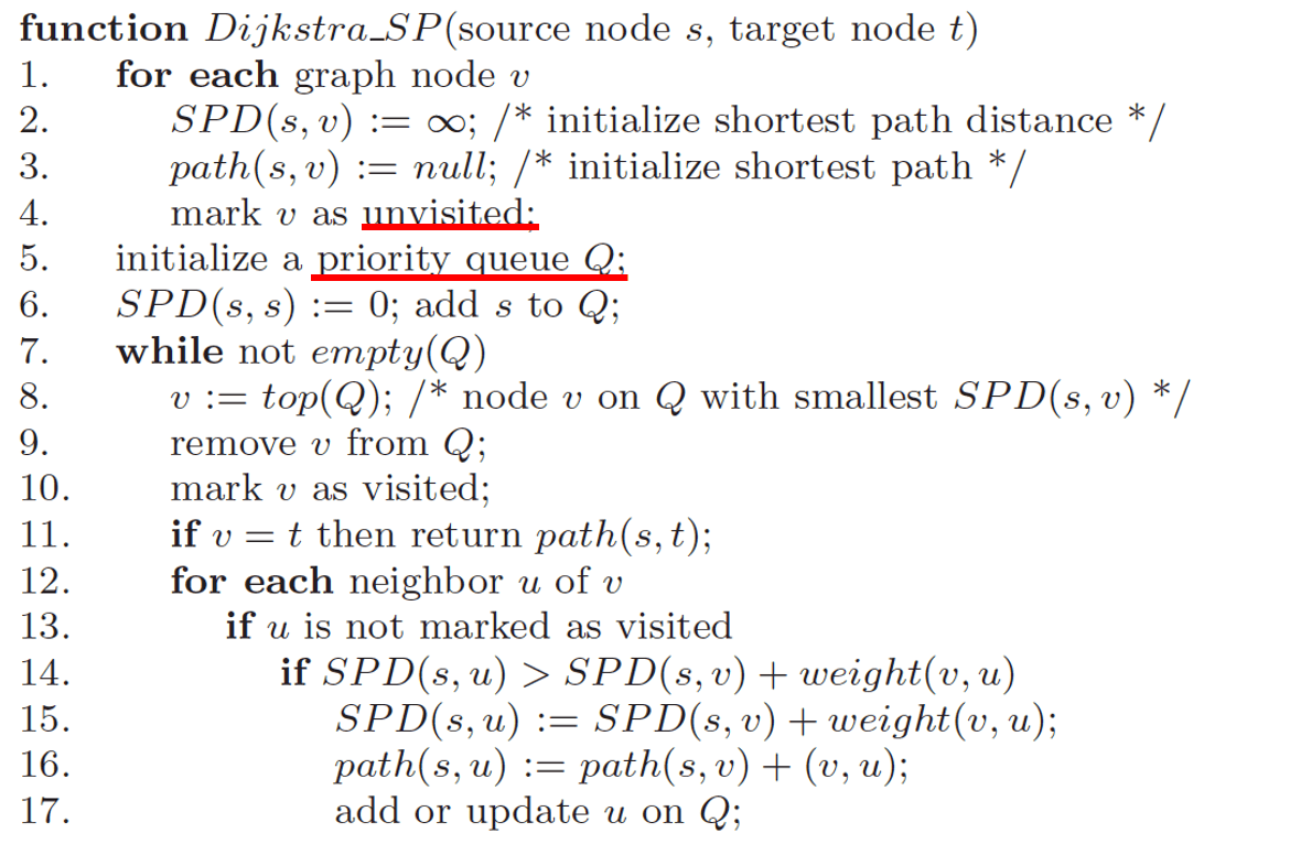
Example
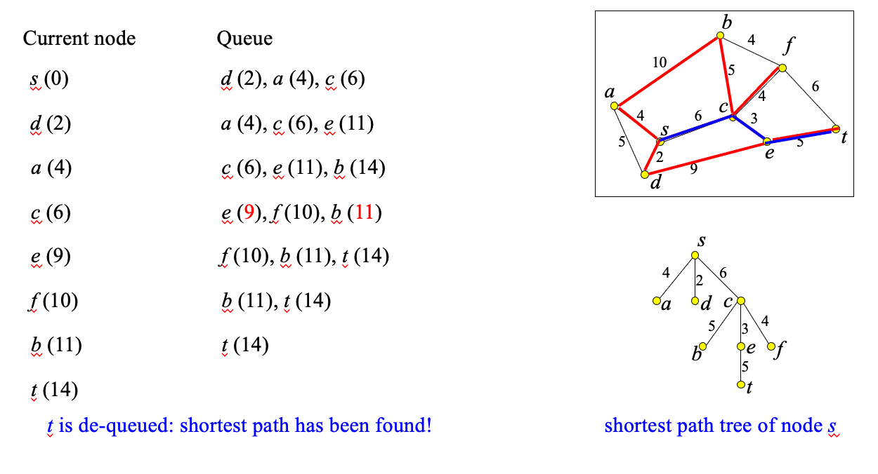
Illustrating
- Find the shortest path between a and b.
- Worst-case performance O(|E| + |V|log|V| )
A*-search
Description
Dijkstra’s search explores nodes around s without a specific search direction until t is found
Idea: improve Dijkstra’s algorithm by directing search towards t
Due to triangular inequality, Euclidean distance is a lower bound of network distance
Use Euclidean distance to lower bound network distance based on known information:
- Nodes are visited in increasing SPD(s,v)+dist(v,t) order
- SPD(s,v): shortest path distance from s to v (computed by Dijkstra)
- dist(v,t): Euclidean distance between v and t
- Original Dijkstra visits nodes in increasing SPD(s,v) order
- Nodes are visited in increasing SPD(s,v)+dist(v,t) order

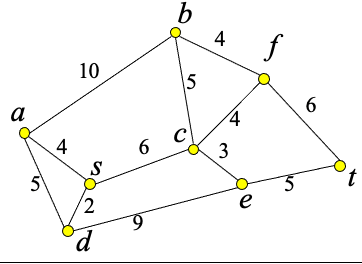
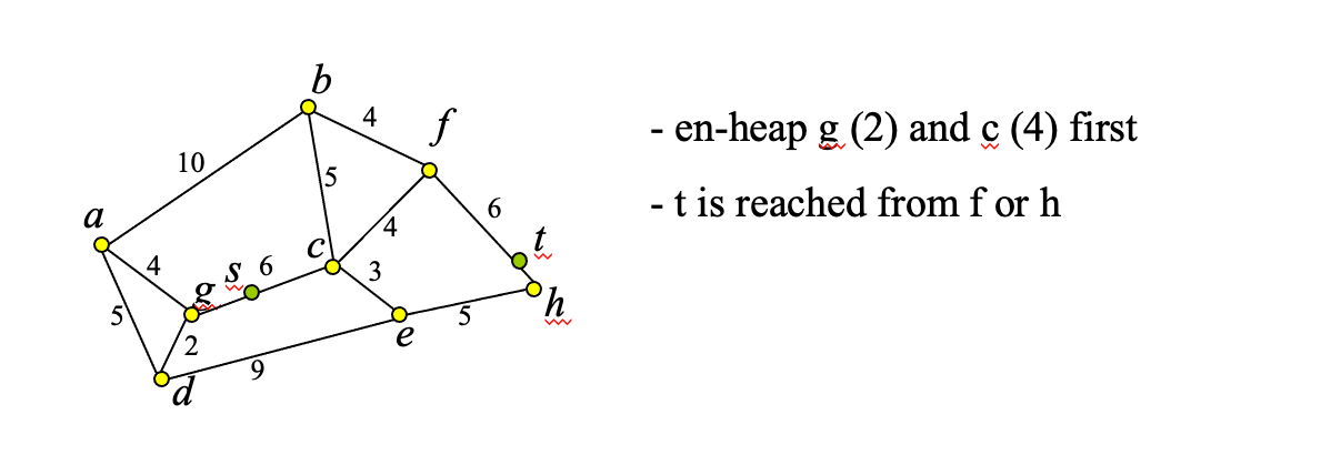
Example

Illustrating
- Find the shortest path between s and t.
- f(p) = Dijkstra_dist(s, p) + Euclidean_dist(p, t)
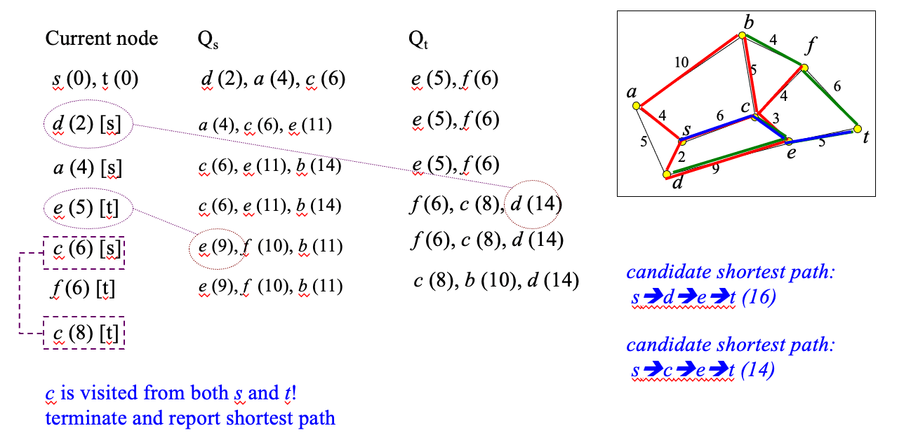
Bi-directional search
- Dijkstra’s search explores nodes around s without a specific search direction until t is found
- Idea: search can be performed concurrently from s and from t (backwards)
- The shortest path tree of s and the (backward) shortest path tree of t are computed in concurrently
- One queue Q_s for forward and one queue Q_t for backward search
- Node visits are prioritized based on min(SPD(s,v), SPD(v,t))
- If v already visited from s and v is in Qt, then candidate shortest path: p(s,v)+p(v,t) (if v already visited from t and v in Q_s symmetric)
- If v is visited by both s and t terminate search; report best candidate shortest path
Example
Discussions
- A* and bi-directional search can be combined to powerful search techniques
- A* can only be applied if lower distance bounds are available
- All versions of Dijkstra’s search require non-negative edge weights
- Bellman-Ford is an algorithm for arbitrary negative edges
Spatial queries over spatial networks
Introduction
Source/Destination on Edges
- We have assumed that points s and t are nodes of the network
- In practice s and t could be arbitrary points on edges
- Mobile user locations
- Solve problem by introducing 2 more nodes
Spatial Queries over Spatial Networks
- Data:
- A (static) spatial network (e.g., city map)
- A (dynamic) set of spatial objects
- Spatial queries based on network distance:
- Selections. Ex: find gas stations within 10km driving distance from here
- Nearest neighbor search. Ex: find k nearest restaurants from present position
- Joins. Ex: find pairs of restaurants and hotels at most 100m from each other
Methodology
- Store (and index) the spatial network
- Graph component (indexes connectivity information)
- Spatial component (indexes coordinates of nodes, edges, etc.)
- Store (and index) the sets of spatial objects
- Ex., one spatial relation for restaurants, one spatial relation for hotels, one relation for mobile users, etc.
- Given a spatial location p, use spatial component of network to find the network edge containing p
- Given a network edge, use network component to traverse neighboring edges
- Given a neighboring edge, use spatial indexes to find objects on them
Evaluation of Spatial Selections (1)
- Query: find all objects in spatial relation R, within network distance ε from location q
- Method:
- Use spatial index of network (R-tree indexing network edges) to find edge n_1n_2, which includes q
- Use adjacency index of network (graph component) and apply Dijkstra’s algorithm to progressively retrieve edges that are within network distance ε from location q
- For all these edges apply a spatial selection on the R-tree that indexes R to find the results
Example
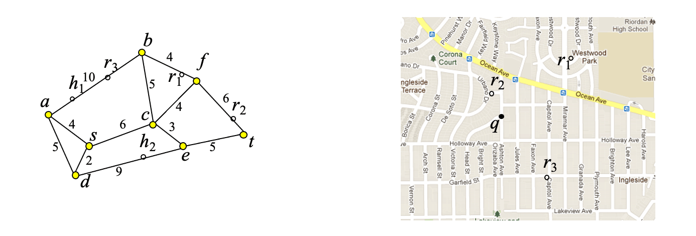
Example: Find restaurants at most distance 10 from q
Step 1: find network edge which contains q
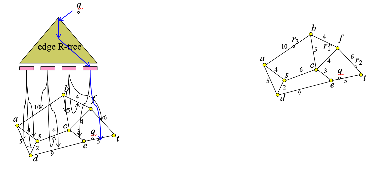
- Step 2: traverse network to find all edges (or parts of them within distance 10 from q)
- Step 3: find restaurants that intersect the subnetwork computed at step 2
Evaluation of Spatial Selections (2)
Description
- Query: find all objects in spatial relation R, within network distance ε from location q
- Alternative method based on Euclidean bounds:
- Assumption: Euclidean distance is a lower-bound of network distance:
- dist(v,u) ≤ SPD(v,u), for any v,u
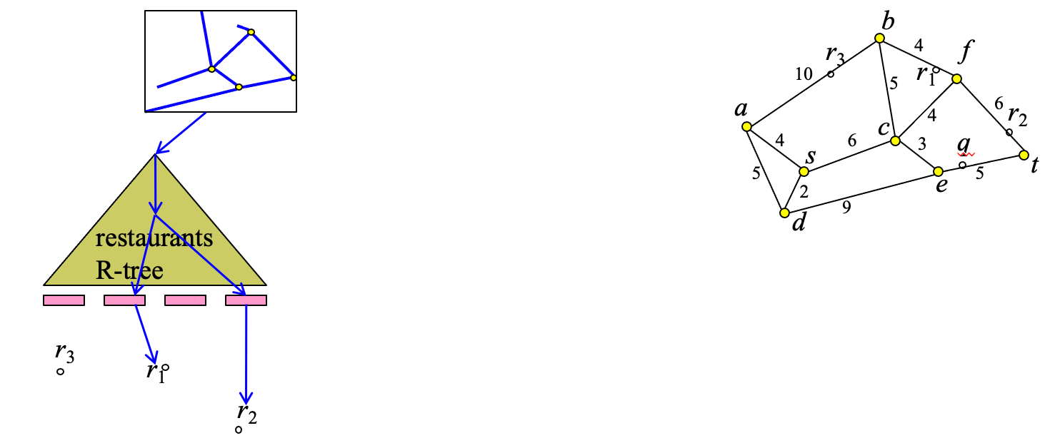
- Use R-tree on R to find set S of objects such that for each o in S: dist(q,o) ≤ ε
- For each o in S:
- find where o is located in the network (use Network R-tree)
- compute SPD(q,o) (e.g. use A*)
- If SPD(q,o) ≤ ε then output o
- Assumption: Euclidean distance is a lower-bound of network distance:
Example
Example: Find restaurants at most distance 10 from q
Step 1: find restaurants for which the Euclidean distance to q is at most 10: S={r1,r2,r3}
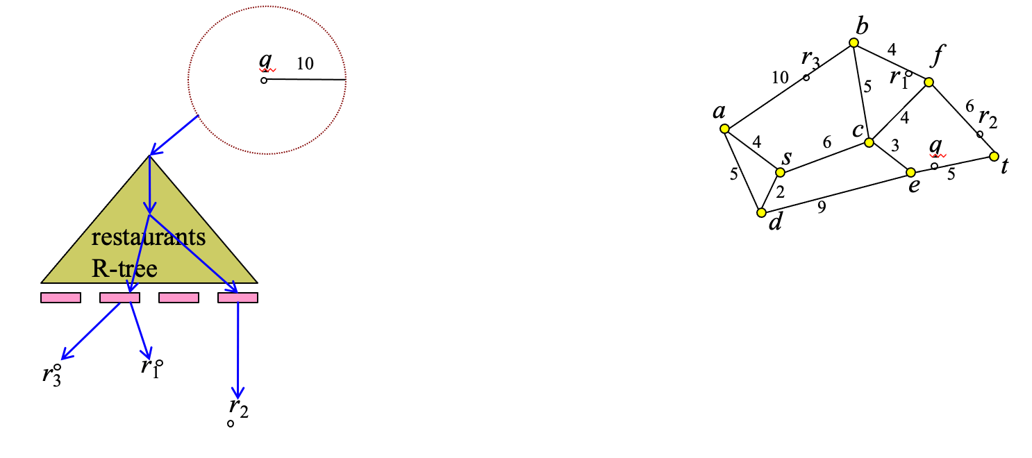
- Step 2: for each restaurant in S, compute SPD to q and verify if it is indeed a correct result
Evaluation of NN search (1)
- Query: find in spatial relation R the nearest object to a given location q
- Method:
- Use spatial index of network (R-tree indexing network edges) to find edge n_1n_2, which includes q
- Use adjacency index of network (graph component) and apply Dijkstra’s algorithm to progressively retrieve edges in order of their distance to q
- For each edge apply a spatial selection on the R-tree that indexes R to find any objects
- Keep track of nearest object found so far; use its shortest path distance to terminate network browsing
Example
- Example: Find nearest restaurant to q
- Step: in ppt 31
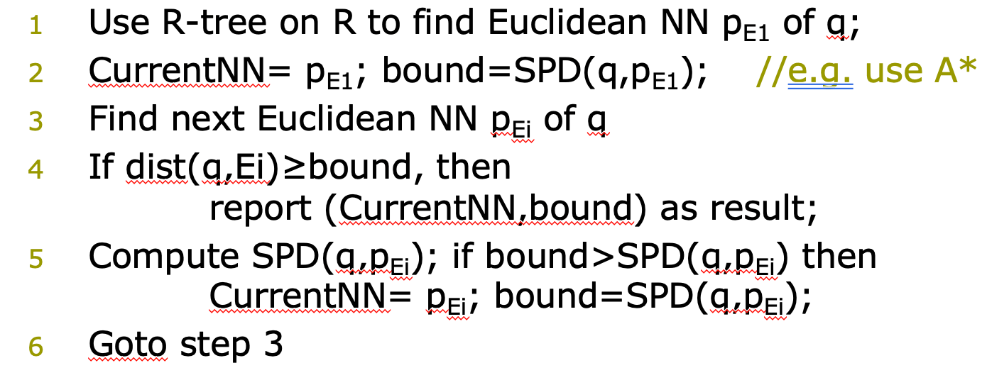
Evaluation of NN search (2)
- Query: find in spatial relation R the nearest object to a given location q
- Alternative method based on Euclidean bounds:
- Assumption: Euclidean distance lower-bounds network distance:
- dist(v,u) ≤ SPD(v,u), for any v,u
- Assumption: Euclidean distance lower-bounds network distance:
Spatial Join Queries
Description
- Query: find pairs (r,s), such that r in relation R, s in relation S, and SPD(r,s)≤ε
- Methods:
- For each r in R, do an ε-distance selection queries for objects in S (Index Nested Loops)
- For each pair (r,s), such that Euclidean dist(r,s)≤ε compute SPD(r,s) and verify SPD(r,s)≤ε
Notes on Query Evaluation based on Network Distance
- For each query type, there are methods based on network browsing and methods based on Euclidean bounds
- Network browsing methods are fast if network edges are densely populated with points of interest
- A limited network traversal can find the result fast
- Methods based on Euclidean bounds are good if the searched POIs are sparsely distributed in the network
- Few verifications with exact SP searches are required
- Directed SP search (e.g. using A*) avoids visiting empty parts of the network
Advanced indexing techniques for spatial networks
Shortest Path Materialization and Indexing in Large Graphs
- Dijkstra’s algorithm and related methods could be very expensive on very large graphs
- (Partial) materialization of shortest paths in static graphs can accelerate search
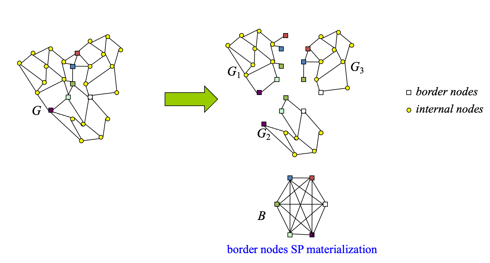
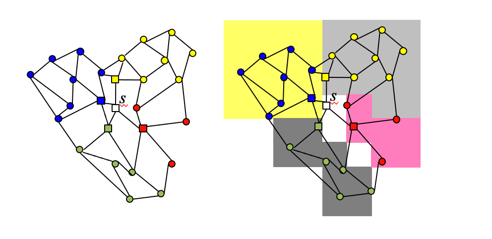
Hierarchical Path Materialization
- Idea: Partition graph G into G_1,G_2,G_3,… based on connectivity and proximity of nodes
- Every edge of G goes to exactly one G_i
- Border nodes belong to more than one G_i’s
- For each G_i compute and materialize SPs between every pair of nodes in G_i (matrix M_i)
- Partitions are small enough for materialization space overhead to be low
- Compute and materialize SPs between every pair of border nodes (matrix B)
- If border nodes too many, hierarchically partition them into 2nd-level partitions
algorithm
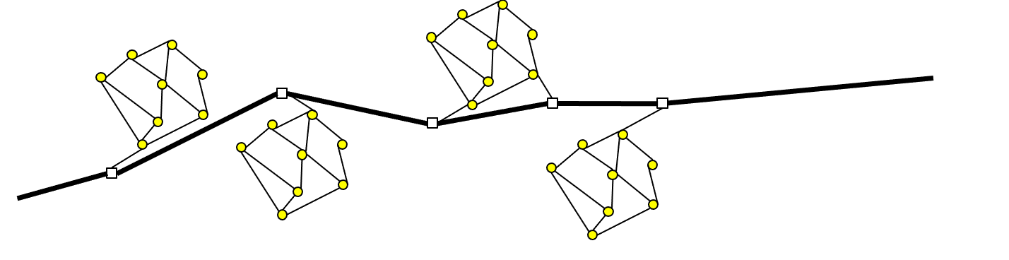
Illustrating
- Good partitioning if:
- small partitions
- few combinations examined for SP search
- Real road networks:
- Non-highway nodes in local partitions
- Highway nodes become border nodes
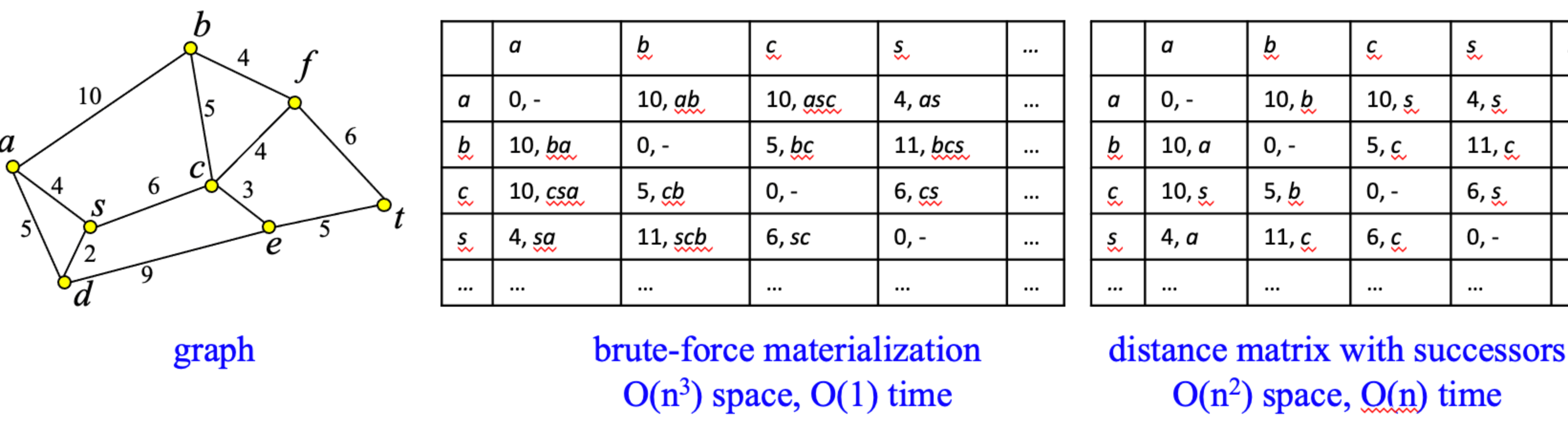
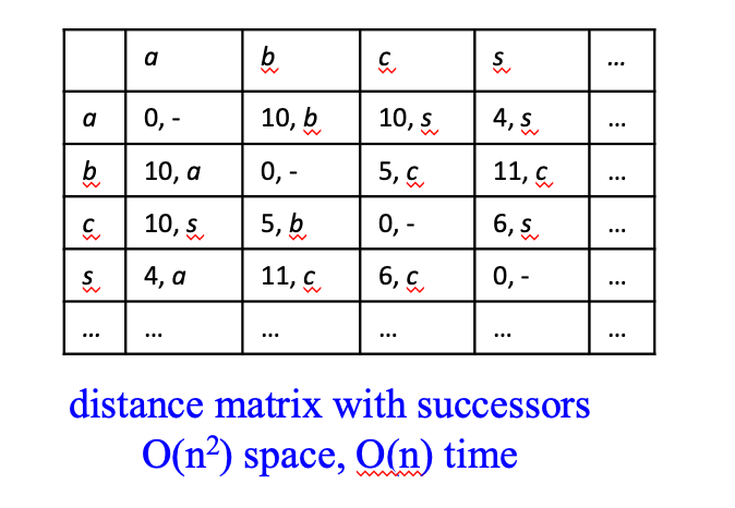
Compressing Materialized Paths
- Distance matrix with successors has O(n_2) space cost
- Motivation: reduce space by grouping targets based on common successors
algorithm
- Create and encode one space partitioning defined by targets of the same successor
- For each node s, index Is a set of <succ,R> pairs:
- succ: a successor of s
- R: a continuous region, such that for each t in R, the successor of s in SP(s,t) is succ
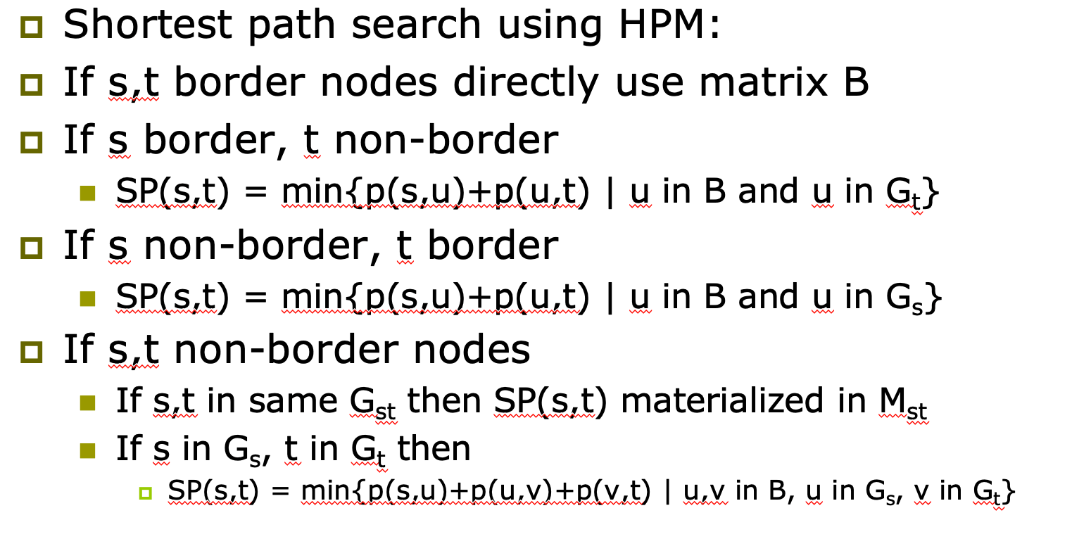
- To compute SP(s,t) for a given s, t:
- SP=s
- Use spatial index Is to find <succ,R>, such that t in R
- SP = SP + (s,succ)
- If succ = t, report SP and terminate
- Otherwise s=succ; Goto step 2
Summary
- Indexing and search of spatial networks is different than spatial indexing
- Shortest path distance is used instead of Euclidean distance, to define range queries, nearest neighbor search, and spatial joins
- Spatial networks could be too large to fit in memory
- Disk-based index for adjacency lists is used
- Several shortest path algorithms
- Spatial queries can be evaluated using Euclidean bounds
- Advanced indexing methods for shortest path search on large graphs
Related Posts

Comments